Manufacturers need to continuously tweak and evolve their fabrication processes to reduce the cost of quality of their products. However, in the process, they often end up introducing new types of defects in products that were not encountered earlier. What can manufacturers do to address this?
Manual Inspection:
This ensures new defects are captured accurately, but it is not scalable. Also, human error around misrepresentation of defects is possible.
Precision Measurements:
These utilize statistical process control and scale well, but are tuned to trigger alerts only on well-studied (known) error types – they’re not effective for novel defects.
Machine Vision Systems:
When trained to detect certain defect types, they scale the best to detect defects on products as soon as they leave the assembly line. But, they’ve traditionally struggled to detect unknown defects.
Approach to Detecting Novel Defects
Recent advances in deep learning have now enabled us to detect such novel defects in real-time. In this article, we outline a new-age approach to detect novel defects in products. Our approach differs from a typical deep learning model development framework in the following stages:
1. Data Collection
Any product has precisely defined dimensions with specified tolerances. Any deviation from this needs to be highlighted as a new defect. To accurately model the specifications, we generate synthetic data to train models. We model the product in a 3D modeling software and programmatically subject the images to a breadth of variations that are typically observed on the production line. We test the effect of each class of data synthesis against a real-world validation set to ensure generalization.
2. Model Selection & Training
Commonly-used best-in-class deep learning algorithms struggle to generalize from synthetic to real-world images. We made significant configuration changes (e.g., introducing normalization, modifying filter configurations, pre-training filters) to achieve that.
We used a Generator–Discriminator (Generative Adversarial Network) structure to discriminate defects from a typical specification. The generator looks to synthesize new images based on a seed, and the discriminator tries to distinguish real from the synthetic images. On training, the generator creates realistic orientations of the product when fed with seeds. And the discriminator generates a confidence score capable of accurately quantifying membership to the training set.
While making determinations on the production line, we traverse a randomly initiated seed vector down the steepest descent to arrive at the minimum in discriminatory error space. This gives us the orientation and form of synthetic image closest to the one seen on the production line.
3. Validation
We carefully curated real-world images for validation purposes. We used the performance measures captured in each set to make model configuration changes, and also training set enhancements.
Example
To illustrate the working of the model, we model a bottle cap as a semi-capsule with a notch using a 3D modeling tool. We subject this shape to a constant illumination and rotate it about a randomly chosen plane to create a large training sample. See Fig 1.

Fig 1. Creating Synthetic Data
To test the performance of the solution, we created two defective samples. One that had a bulge on top and the second with a shortened notch size. The case with a bulge on top is easier to spot manually, while a good solution would be able to capture the second as well accurately. See Fig 2.

Fig. 2. Defective Products
We do not consider surface and texture defects as part of this solution, as specialized procedures exist to capture defects in such cases.
Option 1
The first step towards identifying novel defects is to create a representation of the object. A volume of “True” images in this representational space would be the no-defect set, while cases that lie away from this set would be the defective ones.
To build a representation of the image, we used a UNET. The UNET, in this case, does not employ cross-connections, ensuring that the image descriptor completely describes the relevant components of the image. The convolution layers used a 5X5 filter with a Leaky ReLU and Batch normalization. See Fig 3.
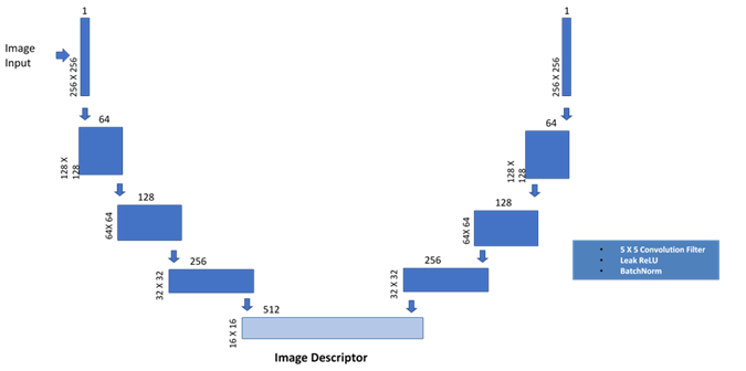
Fig. 3. Architecture of UNET utilized
Training the anomaly detection involves propagating reconstruction error to learn filter weights and separately training a self-organizing map (SOM) on the image description. The SOM learns representations seen during the training phase and recreates the object nearest to the one passed at detection time. See Fig 4.
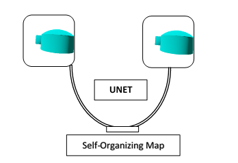
Fig. 4. Architecture of Anomaly Detection using the UNET
We observed two issues with this approach:
1. Learning was hindered in the UNET, so, this approach would not accurately recreate the image as gradients diminished through the filter bank layers. While this may be alleviated through residual connections, we needed a more robust technique.
2. A self-organizing map or other density-based clustering methods introduce additional training and detection time without necessarily improving novelty detection ability.
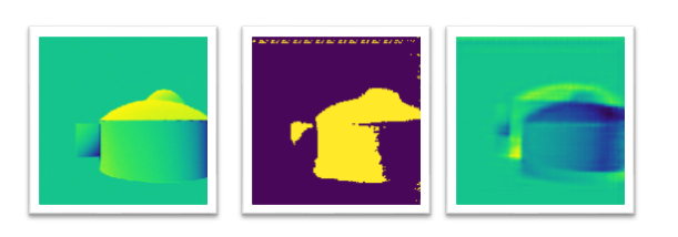
Fig. 5. Results from UNET detection on defect. (Left to Right) Defective input image – Areas reconstructed confidently by the network – Reconstruction error on the defective image
Option 2
An alternative approach is to train the same UNET employing a generator-discriminator framework. The generator helps map points in the image descriptor space to images that mimic real training images. The discriminator trains the encoding filter banks to suppress features uncharacteristic in training images. The two training signals, working in conjunction, effectively train the network to create a representative image descriptor and recreate based on a seen training image.
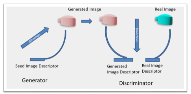
Fig. 6. GAN training: Generator and Discriminator work in tandem to sensitize filter banks to features characteristic in real images
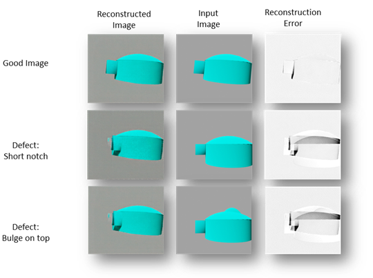
Fig. 7. GAN Reconstruction error
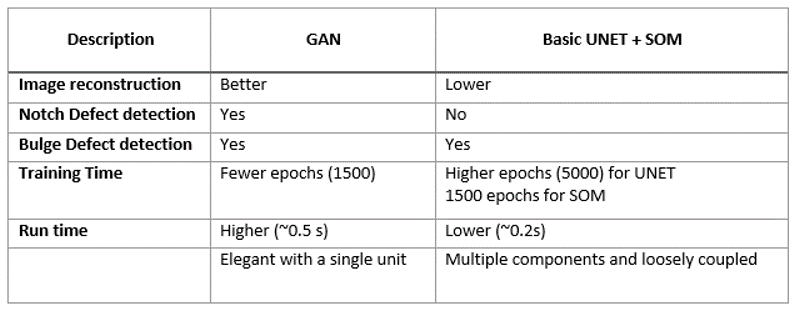
Compared with training a UNET end to end, the GAN can reconstruct the real image with greater ability and alleviates the need for a separate clustering mechanism to locate the nearest descriptor. In the GAN, this search is replaced with elegant gradient descent.
Conclusion
We used manually inspected product samples to measure model performance across broad defect classes. The model performed accurately in identifying novel defect types and post-processing enables localizing the affected component in the assembly. This ability hinges around the number of gradient descent iterations that are performed at detection time, as discussed in the novelty identification stage in our solution section above.
On an average, the model is able to identify a defective bottle cap and localize the affected sub-component in 0.5 seconds, while a good product took 0.2 seconds to pass through using a TensorFlow backend on a GTX 1080 Ti GPU. Scaling this to run real-time would need computation parallelism.
To know more or see a demo, write to info@tigeranalytics.com.
